The quintessential San Francisco resident sits at home hunched over their glowing keyboard and fingerprinted screen, reclined in their thrifted mid century chaise pondering the perils of the market economy. They lift a single blind in their blurple-pastel Victorian's front window and peer out upon the street awaiting the next marginal street infraction. The sash of the aforementioned window is adorned with an intricate z-axis protruding and gilded pseudo-geometric pattern, fastidiously plastered and painted by an unnamed approved artisan with knowledge of old world fabrication techniques. Just above the sash lies a carved x-axis semielliptical alcove with alternating rounded triangular yellow & orange slats depicting a sense of optimism about the sun emerging from the early morning fog laden landscape. The glass suspended in place reflects iridescent hued light from its bubbling manufacturing imperfections when compared to your standard issue insulated double-hung, dual pane modern counterpart. It's this humble threshold at the intersection of past and present where the organic to inorganic proverbial rubicon gets crossed, and grey matter transforms into thumb gestures, into localized machine code, into 5 GHz radio waves, into subterranean server farm machine code and data is manifested into existence from nothingness for better or worse. Plush lounge chair reported infractions range from blight, to 💩, to graffiti, to a personal favorite, pedantic parking violations of all kinds. The SF 311 system retains the culmination of all these reports. It's one glorious dataset that reflects the multitudes of the city I call home. The dataset is available for public download along with a treasure trove of other municipal and election data, nothing less than the city built on the data mined from uninformed consent deserves.

Dataset syncing

With oleander, ingesting this ~5 GB dataset into our Iceberg catalog is pretty simple. Just fire up the oleander CLI and write a simple DuckDB query to extract the .csv file into the system and wait a few minutes looking out the window for no good.

oleander duckdb

CREATE TABLE sf_311 AS
SELECT *
FROM read_csv_auto('311_Cases_20260305.csv');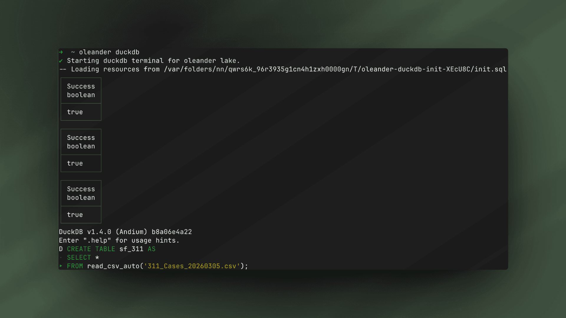

Having this dataset is great, but we also wish to join it with the district populations and demographic data released by the city which is unfortunately only available as html here. I would have given up upon this task yesteryear due to my non-existent attention span that has atrophied due to advent of short form video and my insatiable need for instant gratification, but now I can just Ask AI and have this magically transformed into an insertion statement with ease. This time we'll use the oleander lake to do this instead of the CLI.

INSERT INTO oleander.sf.district_resolution_rate (district, total, closed, closure_rate_pct, run_id) VALUES
(1, 67890, -2722, '85.9%', '-4.0%'),
(2, 70713, 101, '91.9%', '0.1%'),
(3, 65171, -5441, '91.0%', '-7.7%'),
(4, 70672, 60, '83.6%', '0.1%'),
(5, 69278, -1334, '90.1%', '-1.9%'),
(6, 75131, 4519, '90.2%', '6.4%'),
(7, 70793, 181, '84.1%', '0.3%'),
(8, 61483, -9129, '91.3%', '-12.9%'),
(9, 67329, -3283, '81.5%', '-4.7%'),
(10, 77915, 7303, '74.5%', '10.3%'),
(11, 80358, 9746, '79.1%', '13.8%');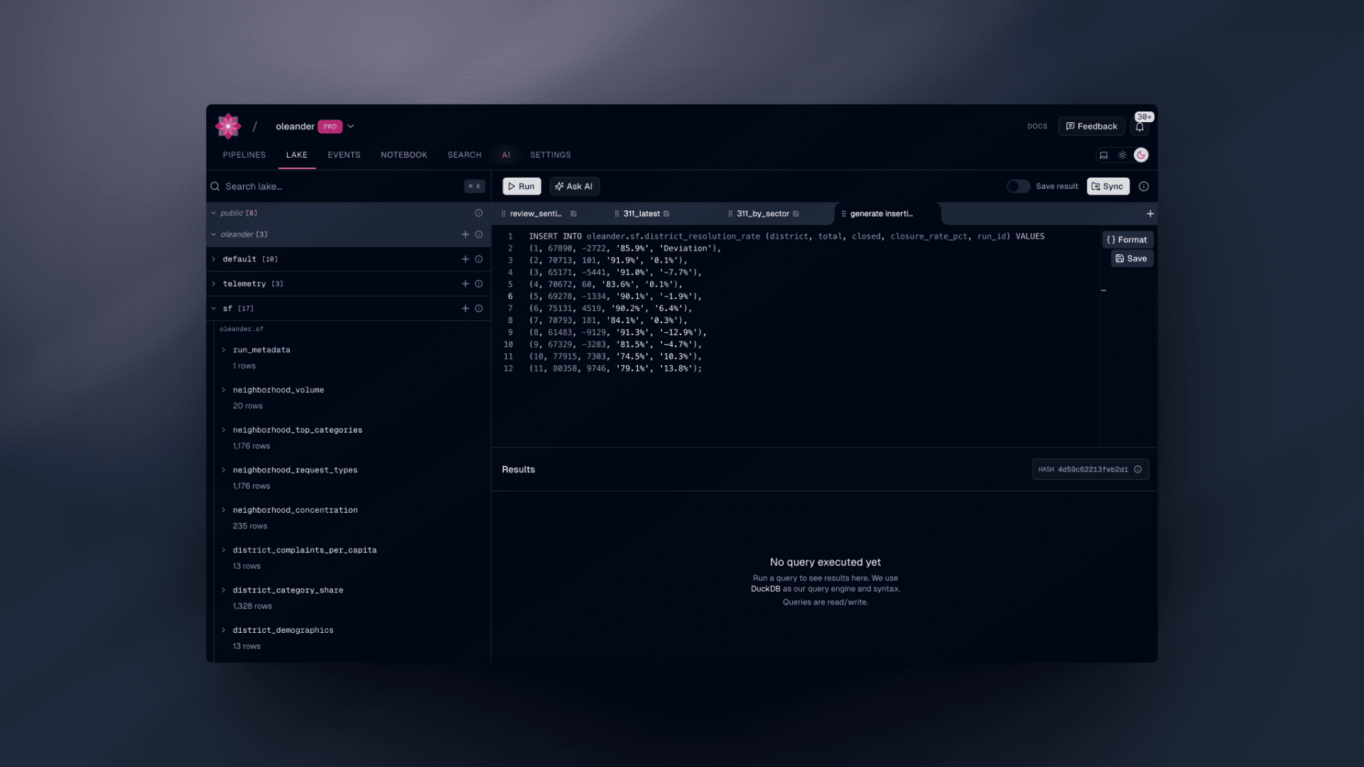

This dataset is now available in the lake for use as is, but also as a Spark input alongside sf_311, which we can use to materialize a more palatable set of derived tables joined with sf_districts. The job itself emits neighborhood concentration metrics, district demographic rollups, temporal breakdowns, and resolution-time summaries back into the Iceberg catalog we came from under new tables.

oleander spark jobs upload ./spark/jobs/neighborhood_stats.py

oleander spark jobs submit neighborhood_stats.py \
  --namespace san_francisco \
  --name sf-neighborhood-stats \
  --wait \
  --args "--top-k 15 --output-catalog oleander.sf"

# spark/jobs/neighborhood_stats.py

SF_311_TABLE = "oleander.default.sf_311"
SF_DISTRICTS_TABLE = "oleander.default.sf_districts"

def _qual(output_catalog: str, table_prefix: str, name: str) -> str:
    return f"{output_catalog}.{table_prefix}{name}"

spark = SparkSession.builder.appName("sf-neighborhood-stats").getOrCreate()
df_311 = spark.table(SF_311_TABLE)
df_districts = spark.table(SF_DISTRICTS_TABLE)

district_counts = (
    df_311.withColumn("district", F.col("Supervisor District").cast("int"))
    .groupBy("district")
    .agg(F.count("*").alias("total_complaints"))
)

district_demographics = (
    district_counts
    .join(
        df_districts.select(
            F.col("DISTRICT").alias("district"),
            F.col("Total_Population").alias("total_population"),
            F.col("Percent_Latino").alias("pct_latino"),
            F.col("Percent_NL_White").alias("pct_white"),
            F.col("Percent_NL_Black").alias("pct_black"),
            F.col("Percent_NL_Asian").alias("pct_asian"),
        ),
        on="district",
        how="left",
    )
    .withColumn(
        "complaints_per_1k_pop",
        F.round(F.col("total_complaints") / F.col("total_population") * 1000, 2),
    )
    .withColumn("run_id", F.lit(run_id))
)

district_demographics.write.mode("overwrite").saveAsTable(
    _qual("oleander.sf", "", "district_demographics")
)

Monitoring your job

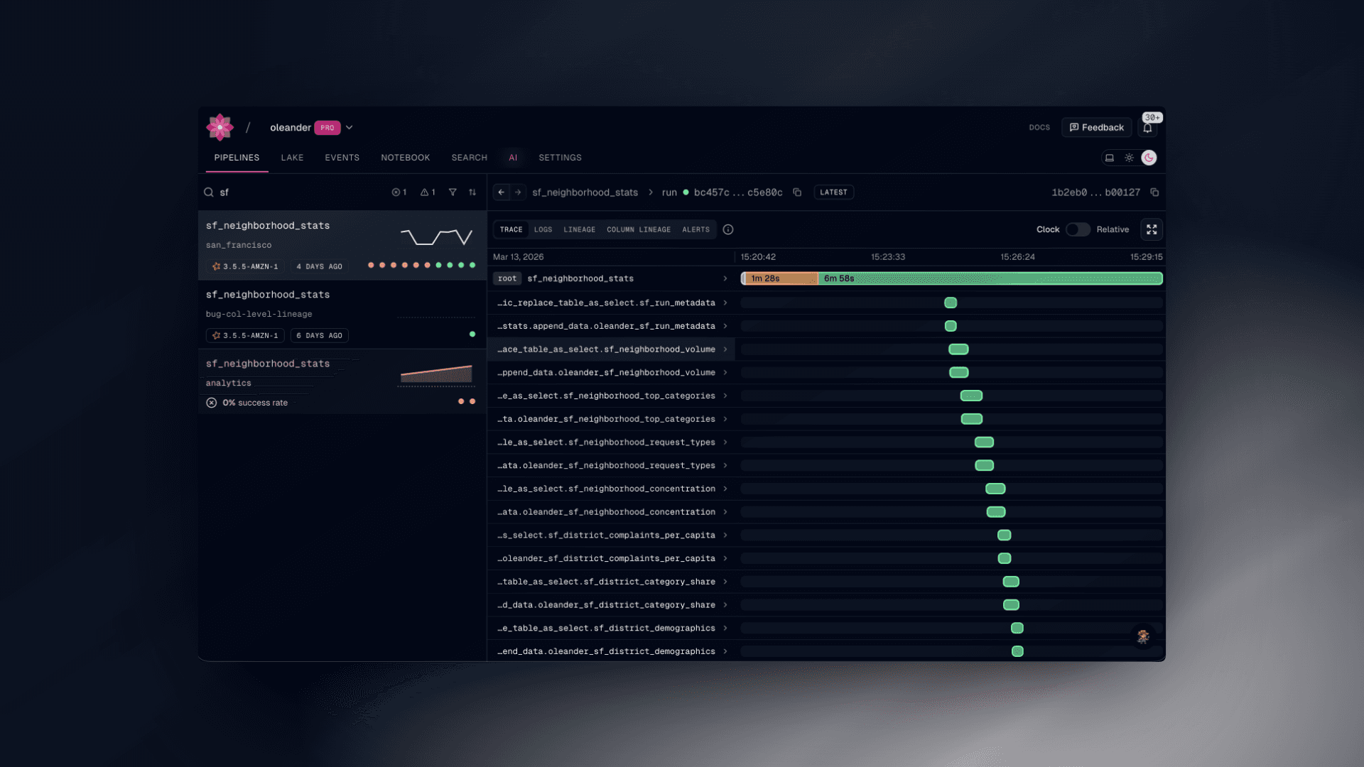
We have finally reached the observability side of the house. We can see the progress of the various functions and logs that the spark task generates during the run sequence. Any error or anomaly that is detected can notify you (or your AI system of choice) a plethora of context to assist with debugging and get you up and running again as fast as possible. Often, in tandem with our MCP server, we’re capable of diagnosing, fixing, and deploying a fix in under a minute.

The future is yours

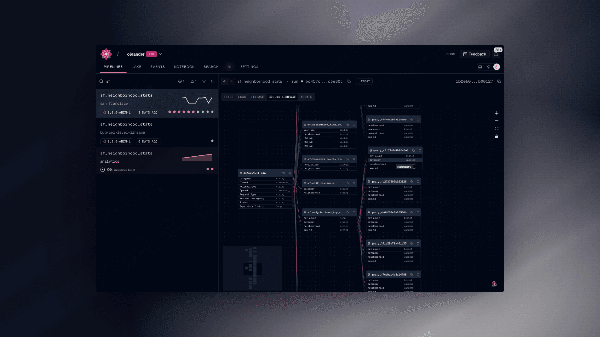
The resulting tables are now available in our lake for arbitrary queries alongside the original tables we used to derive them from. Once we are happy with our Spark task, one possible next step to take is to schedule task runs periodically to generate up to date tables. Of course, since we use Iceberg as our catalog, you can time travel across these historical datasets generated for all of history. Any query that you subsequently run on tables will have table and column lineage captured so that you can experiment with total impunity. Want to run a query correlating complaint density with the slope of the hill? Well you're missing some geospatial data, but you’re already more than halfway there.